Determining a Schwarzschild
Force Function

It’s well known that Newton’s gravity equation does a good job in predicting the motion of objects about large masses, particularly for planets and satellites. It’s also acknowledged that the equation is less than perfect as it fails to properly account for elliptical motion and the path of photons. In such situations one needs to turn to the Schwarzschild metric. This is an equation that predicts motion according to the description of gravity given by General Relativity.

A big problem with the Schwarzschild metric is that applying it is by no means easy. It often involves ‘Lagrangian principles’ and differential equations that can only be solved by approximate means. As such it is normally only used for simple situations.

Newton’s equation by comparison comes in a convenient force form that allows us to determine the net force on a particle. From this we can determine acceleration, i.e. an increase in velocity at any point in time, and hence where a body will be located a short while later. When many bodies are involved such forces can certainly be complicated. But with modern computers this is no problem at all. Instead we can use computers to run accurate simulations telling us for example how planets will move through the solar system, without needing to worry about difficult differential equations.

For this reason it would be helpful to have a way of expressing the metric as a force function rather than the form it’s in. For some reason this function is difficult to find on the internet. There is a reference here [1]. But it gives completely wrong predictions and becomes infinite when orbital velocity is zero.

So this paper will be dedicated to determining a ‘Schwarzschild Force Function’. It will show a derivation from the metric and be followed by computer simulation examples to demonstrate its accuracy.

The Schwarzschild Metric

The first step is to derive a general force function for ‘regular’ bodies (non-photons). This is pretty complex so feel free to skip to the answer (equation 13).

The Schwarzschild metric has the form:

$c^2\text{d$\tau $}^2=\left(1-\frac{\alpha }{r}\right)c^2\text{dt}^2-\frac{\text{dr}^2}{1-\alpha /r}-r^2\sin ^2\theta \text{d$\theta $}^2-r^2\text{d$\phi $}^2$ (1)

Where:
dτ = increment of ‘proper’ (dilated) time
dt = increment of ‘local’ (non-dilated) time
r = radial distance from body being orbited
α (alpha) = the ‘Schwarzschild radius’ = 2GM/c²
M = mass of body being orbited
θ = angle above the x-y plane
φ (phi) = angle on the x-y plane

Consider the case of a test particle (a body much lighter than the central mass M) orbiting on the x-y plane. In this case θ=0, and we can write:

$c^2\text{d$\tau $}^2=\left(1-\frac{\alpha }{r}\right)c^2\text{dt}^2-\frac{\text{dr}^2}{1-\alpha /r}-r^2\text{d$\phi $}^2$ (2)

There are two constants of motion to consider. The first represents angular momentum h:

$h=r^2 \frac{\text{d$\phi $}}{\text{d$\tau $}}$ (3)

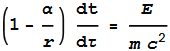
In fact this is angular momentum divided by mass, but if the mass of the particle is constant h will also be constant. The other is total Energy E as derived here [2]:

$\left(1-\frac{\alpha }{r}\right)\frac{\text{dt}}{\text{d$\tau $}}=\frac{E}{m c^2}$ (4)

Start by dividing both sides of (2) by dτ²:

$c^2=\left(1-\frac{\alpha }{r}\right)c^2\frac{\text{dt}^2}{\text{d$\tau $}^2}-\frac{1}{1-\alpha /r}\frac{\text{dr}^2}{\text{d$\tau $}^2}-r^2\frac{\text{d$\phi $}^2}{\text{d$\tau $}^2}$ (5)

Substitute in (3) and write dr/dτ as (r-dot=radial velocity):

$c^2=\left(1-\frac{\alpha }{r}\right)c^2\frac{\text{dt}^2}{\text{d$\tau $}^2}-\frac{1}{1-\alpha /r}\dot{r}^2-\frac{h^2}{r^2}$ (6)

Multiply both sides by (1-α/r):

$\left(1-\frac{\alpha }{r}\right)c^2=\left(1-\frac{\alpha }{r}\right)^2\frac{\text{dt}^2}{\text{d$\tau $}^2}c^2-\dot{r}^2-\left(1-\frac{\alpha }{r}\right)\frac{h^2}{r^2}$ (7)

Substitute in (4) and rearrange:

$0=\left(\frac{E}{m c}\right)^2-\dot{r}^2-\left(1-\frac{\alpha }{r}\right)\left(c^2+\frac{h^2}{r^2}\right)$ (8)

Now take the time derivative of both sides (d/dτ):

$(d/d\[Tau])[0 = (E/(m c))^2 - \!$\*OverscriptBox["r", "."]$^2 - (1 - \[Alpha]/r) (c^2 + h^2/r^2)]$

$\Rightarrow 0=0-2\dot{r} \ddot{r}+\frac{d}{\text{d$\tau $}}\left[-c^2-\frac{h^2}{r^2}+\frac{\alpha c^2}{r}+\frac{\alpha h^2}{r^3}\right]$

$\Rightarrow 0=-2\dot{r} \ddot{r}+\frac{2h^2}{r^3}-\frac{\alpha c^2}{r^2}-\frac{3\alpha h^2}{r^4}$ (9)

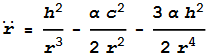
This gives an expression containing radial acceleration (r-double-dot). Now solve for :

$\ddot{r}=\frac{h^2}{r^3}-\frac{\alpha c^2}{2r^2}-\frac{3\alpha h^2}{2r^4}$ (10)

Now substitute in the value for α. Also for the right-hand term, put in h=v_t r, where v_t is tangential velocity, i.e. the velocity at right-angles to the central mass:

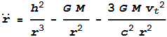$\ddot{r}=\frac{h^2}{r^3}-\frac{G M }{r^2}-\frac{3G M v_t{}^2}{c^2r^2}$ (11)

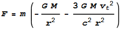
This tells us the total outward acceleration. We know that this will be made up of two components: outward centrifugal force minus inward gravitational force. The centrifugal component is the term on the left: h²/r³, because it is actually v_t²/r. Removing this term and multiplying by small m (the mass of the test particle) gives the gravitational force:

$F=m\left(-\frac{G M }{r^2}-\frac{3G M v_t{}^2}{c^2r^2}\right)$ (12)

This can be more conveniently written:

Schwarzschild Force =

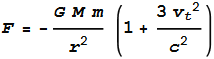$F=-\frac{G M m}{r^2}\left(1+\frac{3 v_t{}^2}{c^2}\right)$ (13)

This is very similar to Newton’s equation except it has an added boost that is in proportion to the square of the orbital velocity. This boost will normally be very small because it’s divided by the speed of light squared.

Testing via Simulation

Now for the fun part. We are going to test this equation using computer simulations. There are various tests that could be done but the best ones are the most famous examples, namely computing the motion of Mercury and the motion of light past the Sun. These will be done using the software Mathematica. For those who have access they can follow the steps and diagrams in this notebook:

download Mathematica notebook

To begin with we’ll look at a simplistic example using exaggerated numbers. Set G=M=m=1. Set the starting position to x=1, y=0; and give the particle an upward starting velocity that will yield an elliptic orbit with eccentricity of 0.7. We’ll also make the speed of light c=10m/s – a very low value because we want the effects to be highly noticeable. This diagram shows the result after 300 seconds:

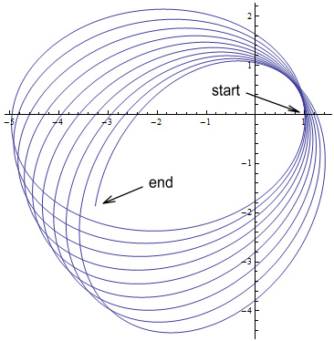
This shows the orbit as a nice ‘Spirograph’ pattern whose elliptic shape remains constant as time progresses. It also shows the precession is in the expected direction (anti-clockwise – same as the orbit direction). So this demonstrates the general concept is correct.

Now consider the real case of Mercury. In this case we predict the precession will be in the same direction although by a much smaller amount.

Before doing this we should specify what we hope for. According to [3] the predicted amount of precession per orbit Ψ is given by this equation:

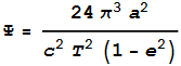$\Psi =\frac{24\pi ^3a^2}{c^2 T^2 \left(1-e^2\right)}$ (14)

Where a is the semi-major axis, T is the orbit period, and e is eccentricity. We would like this in terms of the Sun’s mass and perihelion distance because our simulation will be using that information.

Keplar’s third law of planetary motion tells us that:

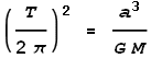$\left(\frac{T}{2 \pi }\right)^2 = \frac{a^3}{G M}$ (15)

And the semi-major axis in terms of perihelion distance r_p is: a=r_p/(1-e). Substituting these into (14) gives:

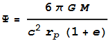$\Psi =\frac{6 \pi G M}{c^2r_p(1+e)}$ (16)

Inserting the values G=6.674x10^-11, M=1.989x10³⁰, c=299792458, r_p=4.600x10¹⁰, e=0.205636, we determine a result of 5.020x10^-7 radians. Converting to arcseconds (multiply by 3600*180/pi) and multiplying by number of orbits per century (415.2) this converts to 43.0 arcseconds per century.

We now apply the same values to a simulation. After one and a quarter orbits, this is what we get:

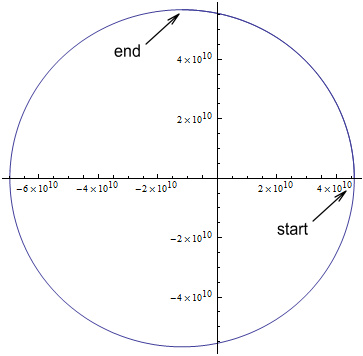
At this scale it’s almost impossible to see any progress. Therefore we’ll instead plot a chart of the outward velocity:

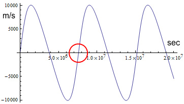
The above graph shows the outward radial velocity of Mercury, i.e. the velocity away from the Sun. When the blue line crosses the x-axis from above that is the aphelion (furthest point of the orbit), and when it crosses from below that is the perihelion (closest point in the orbit).

We need to zoom in on the first perihelion crossover, as indicated by the red circle. Zooming in to a region from 7599356.2031 seconds to 7599356.2033 seconds (two 10-thousandths of a second range), we see the crossover occur at 7599356.2031 seconds. Notice here the outward velocity is in the order of micrometres per second:

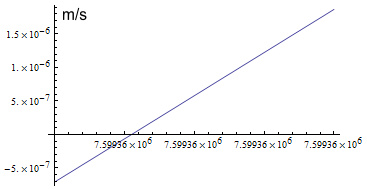
The angle of orbit at this precise point in time is 5.413x10^-7 radians. This equates to 46.4 arcseconds per century.

We were expecting 43 arcseconds so it might appear that the simulation is a bit sloppy. However it needs to be pointed out that the situation is extremely sensitive. If we go back in time to t=7599356.1724 seconds, we get an orbit angle of 5.0196x10^-7 radians, which is the required 43 arcseconds.

This point in time is just 0.03s or three hundredths of a seconds earlier. At that location, just prior to the perihelion point, Mercury is moving toward the Sun at 0.4mm/s and is just 7.6 microns further away!

Dividing 0.03 by t gives a timing error of 4x10^-9 which means we have an inaccuracy just below the 9th significant digit. To overcome this we need to redo the calculation using at least 10 digits of accuracy. Doing so (using “AccuracyGoal->10” in the software) tells us the crossover occurs at t=7599355.6124. This corresponds to an angle of 5.023x10^-7 radians, which works out to 43.02 arcseconds per century – close enough!

So this shows the above ‘Schwarzschild Force’ equation is reliable for predicting advances in elliptic orbits.

Light Bending

Now to perform a similar simulation for the bending of light. It would be tempting to just re-run the above simulation using the same formula and different starting conditions. Unfortunately it’s not that easy because photons have rather different properties to regular bodies. In particular they have zero rest mass while still having finite momentum. So we need to derive a different equation.

Start from equation (8). We are going to replace with an expression in terms of angle:

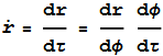$\dot{r}=\frac{\text{dr}}{\text{d$\tau $}}=\frac{\text{dr}}{\text{d$\phi $}}\frac{\text{d$\phi $}}{\text{d$\tau $}}$ (17)

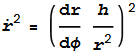
dφ/dτ is the rate of change of angle. This relates to the ‘non-mass angular momentum’ h by h = r² dφ/dτ. So we have:

$\dot{r}^2=\left(\frac{\text{dr}}{\text{d$\phi $}}\frac{h}{r^2}\right)^2$ (18)

Replacing in (8) and dividing both sides by h² gives

$0=\left(\frac{E}{m c}\frac{1}{h}\right)^2-\left(\frac{\text{dr}}{\text{d$\phi $}}\frac{1}{r^2}\right)^2-\left(1-\frac{\alpha }{r}\right)(\left(\frac{c}{h}\right)^2+\frac{1}{r^2})$ (19)

Now replace h with h=L/m, where L is actual angular momentum and m is the mass of the orbiting particle:

$0=\left(\frac{E}{L c}\right)^2-\left(\frac{\text{dr}}{\text{d$\phi $}}\frac{1}{r^2}\right)^2-\left(1-\frac{\alpha }{r}\right)\left(\left(\frac{m c}{L}\right)^2+\frac{1}{r^2}\right)$ (20)

We now set m to zero, or more properly, make it approach zero. Ordinarily this would achieve nothing because angular momentum L would also become zero. But photons are different because they have no rest mass but still have linear and angular momentum. This has the effect of eliminating one of the terms and makes the equation [4]:

$0=\left(\frac{E}{L c}\right)^2-\left(\frac{\text{dr}}{\text{d$\phi $}}\frac{1}{r^2}\right)^2-\left(1-\frac{\alpha }{r}\right)\frac{1}{r^2}$ (21)

Now substitute back in the expression for dr/dφ = r²/h, and we get:

$0=\left(\frac{E}{L c}\right)^2-\left(\frac{\dot{r}}{h}\right)^2-\left(1-\frac{\alpha }{r}\right)\frac{1}{r^2}$ (22)

As before we differentiate both sides by time, and solve for :

$\ddot{r}=\frac{h^2}{r^3}-\frac{3\alpha h^2}{2r^4}=\frac{h^2}{r^3}-\frac{3G M v_t{}^2}{c^2r^2}$ (23)

Converting this to a force equation by removing the centrifugal force term h²/r³ and muliplying by m, we get:

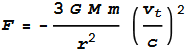$F=-\frac{3G M m}{r^2}\left(\frac{v_t}{c}\right){}^2$ (24)

This is very similar to the earlier expression (13) but without the leading Newtonian gravity term. It seems to be saying: “Light is unaffected by Newtonian gravity and obeys only Einsteinian gravity, whereas regular objects follow both”.

The equation also has the small m in it, but in practice we will ignore that because we are only interested in the acceleration, F/m.

To test this in a simulation, position a small particle on top of the Sun and give it a starting horizontal (tangential) velocity to the right and equal to c:

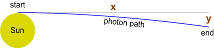
Allowing the particle to move horizontally for a year, it should cover a horizontal distance of one light year. We then need to see how much it falls vertically. The vertical distance in comparison to the horizontal will tell us the deflection angle.

Trying this first using Newtonian gravity tells us the particle moves a horizontal distance of 9.46071x10¹⁵m. This is just under a light-year, which is 9.46073x10¹⁵m, and the slight decrease is due to gravitational pull. The vertical drop is 1.937x10¹⁰m. This corresponds to an angle of 2.047x10^-6 radians or 0.422 arcseconds.

Doing the same for ‘light gravity’ tells us the horizontal distance is almost identical (9.46071x10¹⁵m) and the vertical drop is 3.94438x10¹⁰m. This corresponds to an angle of 4.169x10^-6 radians or 0.860 arcseconds.

In reality the total bending will be double because the particle will curve on both its approach and departure. So we need to double the above numbers to get:

Newtonian prediction: 0.845 arcseconds
Einsteinian prediction: 1.720 arcseconds

So the Einsteinian prediction is just over double the Newtonian.

Out of interest, if we use the earlier Schwarzschild force formula (13) we get 2.595 arcseconds. This is triple the Newtonian and 1.5 times the Einsteinian prediction.

Combining all Methods

For convenience we can construct a combined equation to cover all situations. Specifying two arguments – argN (Newtonian) and argE (Einsteinian) – we write:

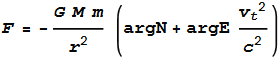$F=-\frac{G M m}{r^2}\left(\text{argN}+\text{argE}\frac{v_t{}^2}{c^2}\right)$ (25)

For classical situations, set:
argN=1 and argE=0

For General Relativity situations, set:
argN=1 and argE=3

For ‘light situations’, set:
argN=0 and argE=3

Tangential velocity v_t can be determined from the relation:

v²=v_t²+v_r²

Where total velocity v is:

v² = v_x²+v_y²+v_z²

and v_x,v_y,v_z are the x/y/z components of velocity. Radial velocity v_r is:

v_r = (x v_x + y v_y + z v_z)/r

To do a simulation then, basically we need to choose a starting position and velocity (in x/y/z components). We then use that to calculate the resulting force (or rather acceleration), split that acceleration into its x/y/z components, and use that to compute an updated position and velocity for a small time-step. We then repeat that over and over and see where the particle goes.

[1] http://www.biblioteca.org.ar/libros/90154.pdf equation 15
[2] https://en.wikipedia.org/wiki/Schwarzschild_geodesics
[3] http://www.math.toronto.edu/~colliand/426_03/Papers03/C_Pollock.pdf equation 42
[4] The logic behind this is questionable because 1/h, and hence m/L, is now hidden within the dr/dφ term, and putting m to zero would make dr/dφ disappear. But that’s the recommended method used here: http://arxiv.org/pdf/0712.3709v1.pdf
, see equation 44

Determining a SchwarzschildForce Function

The Schwarzschild Metric

Testing via Simulation

Light Bending

Combining all Methods

Determining a Schwarzschild
Force Function